In order for us to understand locality sensitive (fuzzy) hashing (LSH), let me take a quick detour via cryptographic hash functions as their features serve as a great explanation for fuzzy hashing.

For a cryptographic hash, two very similar inputs produce two very different hashes. We can simplify this to the statement:

A cryptographic hash function optimizes to avoid hash collisions

A hash collision describes the case were two different inputs result in the same hash. Quite obviously this would be a bad feature for a cryptographic hash used for example to verify the integrity of an input.

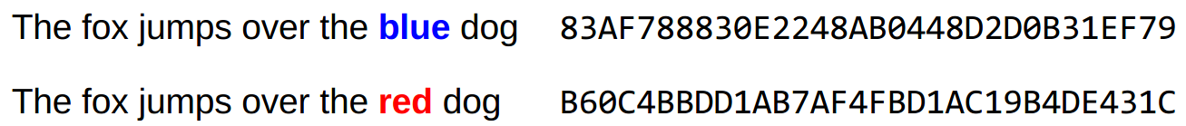Example of a cryptographic hash result

While a cryptographic hash tries to avoid collisions at all costs, a locality sensitive hash tries almost the opposite. While the hash should be different for two distinct inputs, similarities or differences and their location should be represented in the hash. We can simplify this to the statement:

Fuzzy hashing maximizes for partial collision probability

Piece wise Hashing

Piece wise or fuzzy hashing describes the technique where an input is divided into pieces, we calculate the hash for each piece and then use the individual hashes to combine them into the final piece wise result.

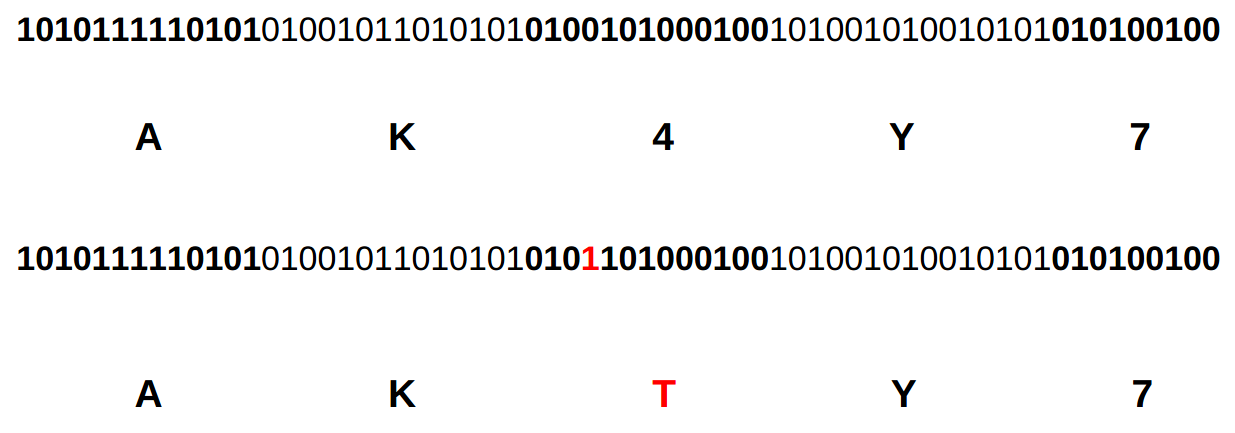Pseudo piece wise hashing

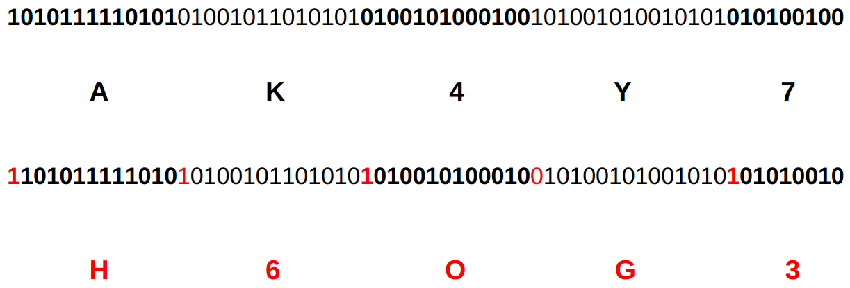
In the above example we calculate the piece wise hash AK4Y7 from the input. We then make a change to the input, resulting in a variation in one of the input pieces, its hash and eventually in the resulting input hash: AKTY7. We could now assume from just looking at the two hashes that the two input files only vary by one piece. This is the core concept of piece wise hashing.

Locality Sensitive Hashing

What we have achieved with the previous example is a reduction in dimensionality. We took the complexity of our input and reduced it to hashes of pieces. Another example of how a hashing algorithm reduces dimensionality is a bloom filter where we reduce complexity at the expense of accuracy. The input data is reduced into buckets.

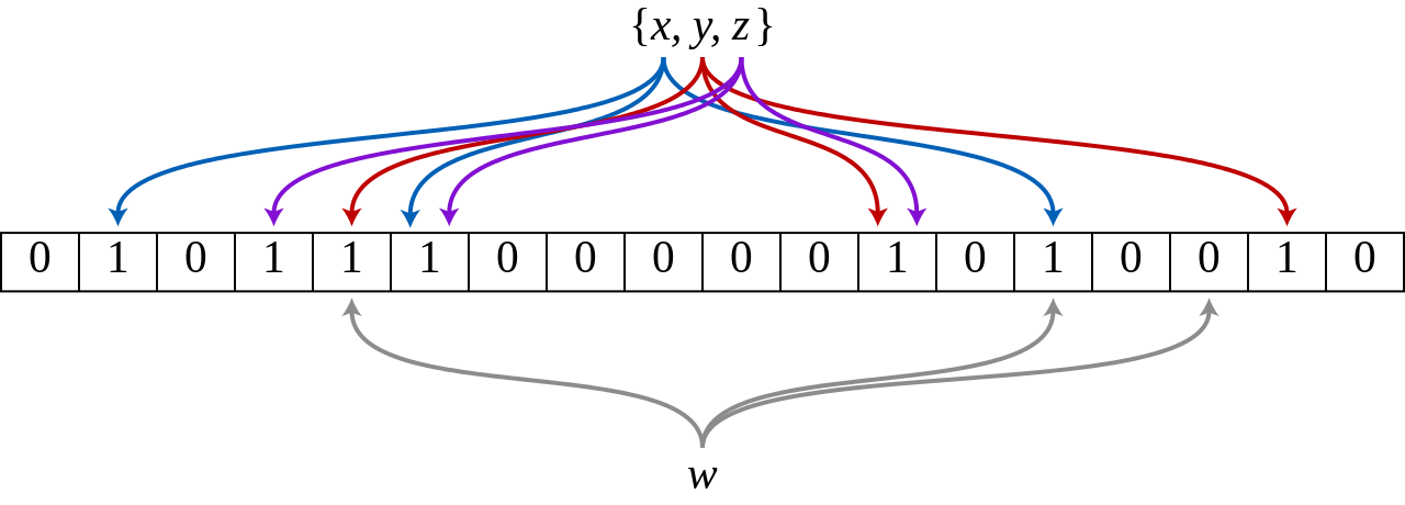Bloom filter: Input data is put into buckets resulting in reduced complexity Source

Another feature resulting from the concatenation of the hashes in the order of the pieces, is the preservation of locality. The result is called a locality sensitive hash.

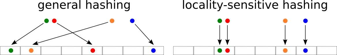Comparison of general hashing with locality-sensitive hashing

As you can tell from this example, the location of the piece in the input file is reflected in the location of the hash of the piece in the input files location sensitive fuzzy hash.

Comparison of fuzzy hash results

With the fuzzy hash at hand, we would like to leverage the optimization towards collisions to use the hashes in order to make a statement about the input files similarity. To do so, and leveraging the locality, we can just hold two hashes next to each other and compare them character by character. The more matches we get, the more similar are the two input files.

Edit distance between two strings Source

The various implementations of fuzzy hashes have slightly different approaches to actually compare two hashes, but in their core they rely on the concept of edit distance. If we use our knowledge so far, we can translate the delete, substitute and insert operations when comparing two hashes easily to changes to our input. Naively the greater the edit distance between two hashes, the less similar are the input files.

Context Triggered Piece-wise Hashing (CTPH)

So far we haven’t really discussed how we would choose the pieces in our piece-wise hashing algorithm. This is actually an interesting problem. Let’s say we split the input into equally length chunks from the start of the input. If we now prepend data to our input, our piece-wise hashing falls apart:

Prepending data to the input offsets all pieces

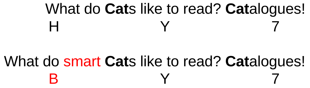
Instead of using fixed length and offset chunks, we could use a context based trigger for the chunk borders. In the following example we are picking the string Cat as trigger for our pieces and hash them as we did before. If we now insert new content into our input, only the hash for the changed piece is affected:

Content triggered piece wise hashing

One of the most prominent implementations of context triggered piece-wise hashing is SSDEEP.

SSDEEP, a CTPH implementation

In order to generate the triggers, SSDEEP uses a rolling hash algorithm producing a pseudo-random value based only on the current context of the input. A sliding window is passed as input and whenever the generated rolling hash matches our trigger, we compute the traditional hash on the current piece. Originating from the spamsum algorithm, SSDEEP uses the term block size for the trigger value.

Initial block size

Where b_min is a constant minimum block size, n the input length in bytes and S the Spamsum minimum length. b_init is called the initial block size as it might get adjustments during the computation of the hash. E.g. if the final hash length doesn’t fulfill the minimal requirements, the block size might be reduced and the hash recalculated. As one can imagine, this is a major performance problem, especially for small files or low entropy files.

Whenever we hit the trigger value with our rolling hash, we have the end of a new piece of data of which we then calculate the Fowler–Noll–Vo (FNV) hash. FNV is not a cryptographic hash but its optimization for hash tables and checksums makes it a great candidate in our application. We then take the base64 encoded value of the the six least significant bits (LS6B) of the FNV hash and appended it to the first part of the final signature.

When comparing two SSDEEP hashes, we start with the block size. We can only compare hashes with identical block size. Next step is the elimination of recurring sequences. Sequences indicate patterns in the input file which hold little information and therefore have insignificant impact on the content. Finally we calculate a weighted edit distance between the two resulting hashes. The edit distance represents the minimal number of mutations required to get from one input to the other. The weights are set to:

SSDEEP hash comparison

The normalized match score represents a conservative weighted percentage of how much two inputs are ordered homologous sequences. Which represents how many of the bits are identical and in the same order. Two dissimilar files can have the same SSDEEP hash if their differences don’t affect the trigger points and the FNV hash is creating a collision in the LS6B. The possibility can be reduced by replacing FNV with a cryptographic hashing algorithm. The reference implementation of SSDEEP can be found on SourceForge and our Go implementation on Github.

Trend Micro Locality Sensitive Hash (TLSH)

TLSH starts off with reading a sliding window over the input file while creating a Pearson Hash. In the below pseudo code of the Pearson hashing algorithm, our window input W of bytes returns a single byte h from a table T with the shuffled values from 0 to 255.

function PearsonHash(W):
  h := 0
  for each b in W:
    h := T[ h XOR b ]
  return h

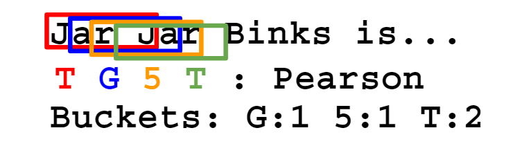
We prepared a range of buckets for all potential Pearson hashes we could observe. We increment the counts of respective buckets creating a frequency distribution. This way we reduce the input complexity using a simple hashing algorithm and by counting frequencies of buckets.

Pearson Buckets

After step 1 has been performed we have an array of bucket counts. We calculate the quartiles of this array such that:

75% of the bucket counts are >= q1
50% of the bucket counts are >= q2
25% of the bucket counts are >= q3

We selected the quartile points rather than the average used by the Nilsimsa hash for a similar purpose to make the scheme work well on binary data such as binary files and on images.

Construct the digest header

The first 3 bytes of the hash define the header. The first byte is a checksum (modulo 256) of the byte string. The second byte is a representation of the logarithm of the byte string length (modulo 256). The third byte is constructed out of two 16 bit quantities derived from the quartiles q1, q2 and q3:

q1_ratio = (q1*100/q3) MOD 16
q2_ratio = (q2*100/q3) MOD 16

We end up with:

header = checksum(bytes) + log(bytes) + q1_ratio + q2_ratio

Construct the digest body

The remainder of the digest is constructed using the bucket arrays values by comparing them to the quartiles q1, q2 and q3. The following simple loop produces the binary representation of the remaining digest.

for i = 0 to 127
  if bucket[i]      <= q1 Emit(00)
  else if bucket[i] <= q2 Emit(01)
  else if bucket[i] <= q3 Emit(10)
  else Emit(11)

The final TLSH digest is constructed by concatenating the hexadecimal representation of the digest header and the binary digest body.

Implementing TLSH in Go

From the very beginning we had a test that compared our libraries output with the reference implementation. While it took some time until we finally passed the test, it was a good feeling having a clear goal and constant confirmation for our progress. Shortly after the first working version, we added Continuous Integration support. Travis was running our test suit on every commit, making sure pull requests never broke functionality.

While pure functionality is a minimal requirement, we early started to also observe the performance. Especially the impact of change. To do so, critical components got Benchmark coverage and it became common practice to compare performance before pushing new code.

We are using a simple make command to create a comparison between the current code changes and the HEAD of the project:

benchcmp: 
  go test -test.benchmem=true -run=NONE -bench=. ./... > curr.test 
  git stash save "stashing for benchcmp" 
  @go test -test.benchmem=true -run=NONE -bench=. ./... > head.test 
  git stash pop 
  benchcmp bench_head.test bench_current.test

Here is a comparison of benchmarks between unrolling a loop in the Pearson hash and our original implementation:

benchmark                     old ns/op     new ns/op     delta
BenchmarkPearson-4            0.29          5.41          +1765.52%
BenchmarkFillBuckets-4        7280          11789         +61.94%
BenchmarkQuartilePoints-4     1805          1846          +2.27%
BenchmarkHash-4               12673         17227         +35.93%
BenchmarkModDiff-4            0.29          0.29          +0.00%
BenchmarkDigestDistance-4     36.3          36.1          -0.55%
BenchmarkDiffTotal-4          43.7          44.2          +1.14%

While this is a drastic example, it is a quite obvious demonstration how quickly things can go bad with just some minor changes.

While there is a reference implementation in C++ available, we had excellent guidance from the original paper. This led to various decisions affecting performance in a positive way without getting to caught up in tedious translation.

Lessons learned

Fuzzy and location sensitive hashes are great tools and by implementing them you will get deep insight into their limitations and strengths. There is no best hashing algorithm in this field and you should make an educated choice or if you have the resources use more than one.

Footnote: The compiler most likely ends up generating better ASM than you…